| Version 2 (modified by varunr, 14 years ago) (diff) |
|---|
8.6 Import time series
There are two main types of data that you can read in to Ecosim: historical comparison data and time forcing data. Historical comparison data enable comparison between historical observations and the model’s predictions. Time forcing data are used to actually force certain variables (fishing effort, fishing mortality) in the model (i.e., ‘drive’ the model). You can load both types of data with the same data file, using the codes for different data types listed below (forcing data types are indicated in parentheses).
The time series data file
For historical comparison data, you can leave cells blank for which you have no data. Ecosim will assume that the first calendar year for which you enter a data row (e.g., 1976) is to be the simulation start year. Forcing time series must have an entry for every year of the simulation. Note that relative fishing rate by gear type must be scaled so relative value is 1.0 for the Ecopath base year (year for which catches are provided to Ecopath).
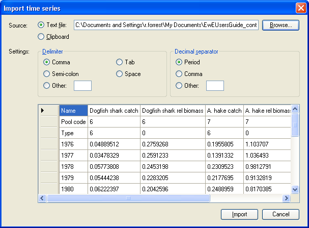
The spreadsheet must be identical in format as shown in Figure 8.8 (i.e., cells 1-3 in the first column must read “Name”, “Pool code” and “Type” respectively and the years of the simulation must be listed below these in the first column). For each data series (column) you must enter the Ecopath group or fleet number (Pool code) and specify the data type (see list of data types below). You can use the first row (Name) to describe the group and the data. This information will be displayed on output graphs.
Optionally, a row labelled “Weight” can be inserted between the name and pool code rows, in which users can specify time series weights. If this row is omitted, time series will be imported with a default weight of 1.
Overview of data types:
-1 Force biomass (forcing)
0 Relative biomass *
1 Absolute biomass
2 Time forcing data (forcing)
3 Effort data by gear type (forcing)
4 Fishing mortality, (F) by pool (forcing)
5 Total mortality, (Z) by pool
-5 Forced total mortality (Z) (forcing)
6 Catches
-6 Forced catches (forcing) †
7 Average weight (stanzas only)
- The software takes the ratio of ‘observed’ to estimated value for the years where there are observations, log it, ln(Oi/Ei?). Then we estimate a scaling factor, S, as, S = exp[sum(ln(Oi/Ei?))/count(i)]. Each of the observations is then plotted on top of the estimated value as Oi / S. (Oi Observed parameter no i, Ei Estimated parameter no i )
Using data type 2, you can force nutrient concentrations (see Ecosim parameters and links therein); parameters that affect trophic interactions through abiotic factors (see Forcing function and Apply FF (consumer)) or primary production (see Apply FF (primary producer)).
† Forcing catches enables Use of Ecosim for Stock Reduction Analysis?.
How to import a time series data file
Important note. After importing a time series file, you must weight the time series using the Time series form.
Note that you must already have an Ecosim scenario loaded before you can import a time series data file (see Ecosim menu? for instructions for creating and loading Ecosim scenarios).
The Import time series dialogue box (Figure 8.8) allows you to load time series data stored in CSV (comma separated values) or similar text format. It can be accessed:
(i) from the Ecosim menu; or
(ii) from the Time series form (Import…).
To read in a data file, click Browse to locate your file or select it from the clipboard. You must then set the delimiter used to separate the values in the csv or text file and the separator used as a decimal point. Your data will be displayed in the bottom window of the form (see Figure 8.8). If everything looks as you expected it, click the Import button. If the data is not displaying as expected, first double-check that the Delimiter and Decimal separator settings are correct before checking that your file is in the correct format.
Figure 8.8. The Import time series dialogue box.
