| Version 2 (modified by shermanl, 13 years ago) (diff) |
|---|
10.6 Dispersal
Introduction
The organisms (i) in an Ecopath model have an aggregated biomass (Bi), and are not assumed to move within the area covered by that Ecopath model. In Ecospace, a fraction (B'i) of the biomass of each cell is always on the move, wherein
B' = m · Bi
with m having the dimension of length / time (i.e., km / year) i.e., a velocity or 'speed'.
However, m is not a rate of directed migration, as occur seasonally in numerous fish populations. Rather, m should be regarded as dispersal and seen as the rate (km/year) the organisms of given ecosystem would disperse as a result of random movements.
Thus, Ecospace simulation are initiated by distributing all organisms evenly onto the basemap, at the density (t · km-2) defined by the underlying Ecopath model. Then all biomass pool start moving, as a function of their value of m, out of their cell and into adjacent cells, there consuming food, and being themselves consumed.
Given differential food consumption and survival rates in preferred vs. non-preferred habitat, this will soon generate richly patterned distributions, wherein each cell includes different biomass of each of the groups in the system.
Note that the final results of Ecopath simulations tend to be largely independent of the specific values of m used, and hence long debates on the best choice of these values may not be necessary - at least not until field estimate, based, e.g., on tagging studies have become available.
Note, finally that the biomass of a group within a given cell is usually not multiplied by the same value of m for each of the flows out of the cell (4 in the case of a cell not touching on land).
Base dispersal rate
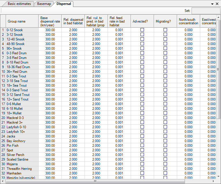
This is the absolute value of m to be used in the simulation. The default value is 300 km/year for all groups apart from detritus groups to which discards are added (and for which we use a default of 10 km/year).
Relative dispersal in bad habitats
The dispersal rates are assumed to differ between preferred and non-preferred habitats, with higher values of m within non-preferred habitats than in preferred habitats. Such assumption is realistic as it implies that organisms in non-preferred habitats will strive to leave these, and attempt to return as rapidly as possible to their preferred habitats.
The default value for the multiplier of m is 2.0 and the upper limit 10.
Vulnerability to predation in bad habitats
The increased vulnerability to predation (or grazing) of various organisms outside their 'preferred' habitat can be changed using a multipliers. The default value of the multiplier is 2.0 for all groups, and it can be increased by up to a factor of 100, while entering a value of 1 will make this mechanism inoperative.
Conceptualizing this mechanism is straightforward: imagine as an extreme case how easy it would be for a pelagic carnivore to grab a typical coral reef fish, e.g. a butterfly fish, blown by a freak wave off its reef, into an open water area. A less extreme case would be a member of a very abundant population, pushed out of its preferred habitat by its competitors of the same species.
To avoid occurrence of groups outside of their preferred habitats you should set the vulnerability to a high value.
Relative feeding rates in bad habitats
Organisms outside their preferred habitat may be conceived as less likely to consume as much appropriate food as their congeners within preferred habitat, due to the unavailability of such food or the danger associated with foraging.
To simulate this, Ecospace users can reduce the feeding rate of ecosystem components down to 0.01 times the Ecopath baseline (i.e., the Q/B value). The default is 0.5, and this mechanism can be made inoperative by setting the feeding rate multiplier equal to unity (1).
Advected?
Indicate here whether a group is advected or not, this may, e.g., be the case for plankton. See Advection for more details on implementing advection in Ecospace.
Migrating?
Indicate here whether a group is migrating or not. For migrating groups/life stages enter concentration parameters and define migration patterns (using the so named button). See Representing seasonal migration in Ecospace for more details on implementation of seasonal migration in Ecospace.
North/south and East/west concentration
Larger organisms commonly have seasonal migration patterns that allow them to utilize favourable seasonal resource and environmental conditions over large spatial areas. Such movements can be represented in Ecospace in two ways. First is a simple “Lagrangian” approach that does not require explicit simulation of movement; the idea here is to simply think of the whole Ecospace map as moving in space so as to remain centred on the distribution of some dominant migratory specie(s). Second is a more complex “Eulerian” approach, which does involve explicitly modelling changes in instantaneous rates of biomass flow among the Ecospace spatial cells, in some way that approximates at least the changing centre of distribution of the migratory species.
The Eulerian approach is implemented in Ecospace by allowing users to define a monthly sequence of “preferred” map cell positions and to define how spread out the migrating fish are likely to be around these preferred cells by setting north-south and east-west “concentration parameters”.
For more detail see Representing seasonal migration in Ecospace.
Barrier avoidance weight
To prevent migrating fish getting stuck in complex habitat, Ecospace contains an algorithm to help fish move around obstacles. The Barrier avoidance weight is the weight placed on the path finding algorithm. Default is 0 (it does nothing). If fish are getting stuck, gradually increase the value up to 1. Increasing this weight tends to concentrate the fish more tightly. The EW/NS concentrations can be lowered if this is a problem.
Figure 10.8 Ecospace dispersal rates and habitat specific information. Migration patterns are also defined on this form.
